Transposing cells in Excel is an easy process of rotating data from rows to columns or vice versa. Here are the simple steps to do it:
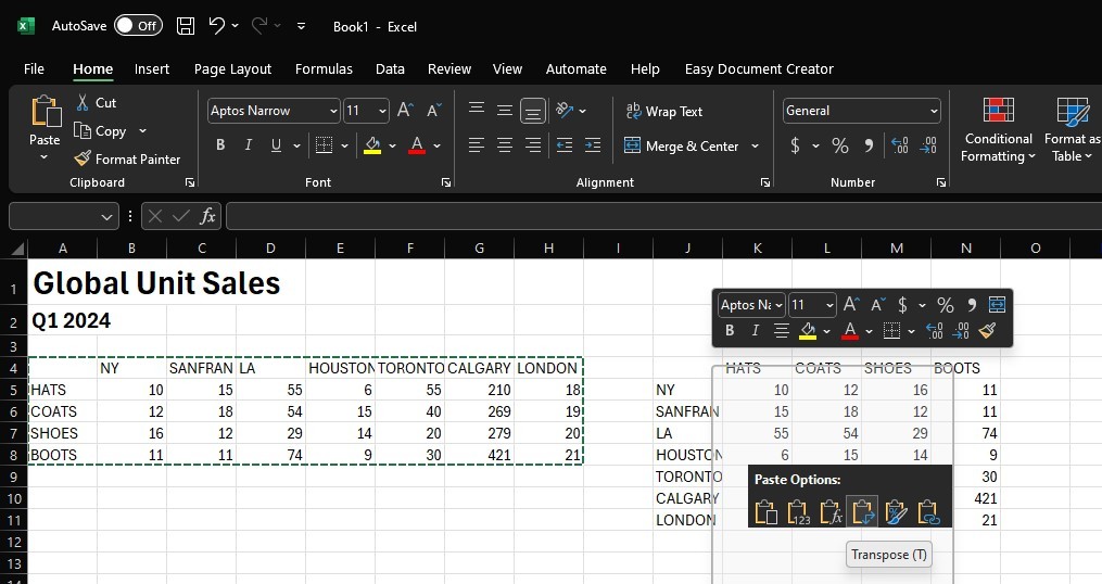
- Copy the cell range: Select the range of data you want to rearrange, including any row or column labels, and or right click and select COPY (or press Ctrl+C).
- Select the empty cells: Choose a new location in the worksheet where you want to paste the transposed data. Make sure there is plenty of room to paste your data. The new table that you paste will overwrite any data or formatting that’s already there.
- Paste “Transpose”: Right-click over the top-left cell of where you want to paste the transposed table, and then choose Transpose under the Paste Options.
The original and the transposed tables are completely unlinked. After rotating the data successfully, you can delete the original table without affecting data in the new table.
Note that if your data includes formulas, Excel automatically updates them to match the new placement. You should verify these formulas use “absolute references“. If they don’t, you can switch between “relative, absolute, and mixed references” before you rotate the data.


0 Comments